d2l 学习记录
数据处理
N维数组
0-d 标量 一个类别
1-d 向量 一个特征向量
2-d 矩阵 一个样本-特征矩阵 每一行表示一个样本,每一列表示一个不同特征
3-d RGB图片
4-d 一个RGB图片批量
5-d 视频
创建数组
创建数组需要三个要素:
形状
数据类型
每个元素的值
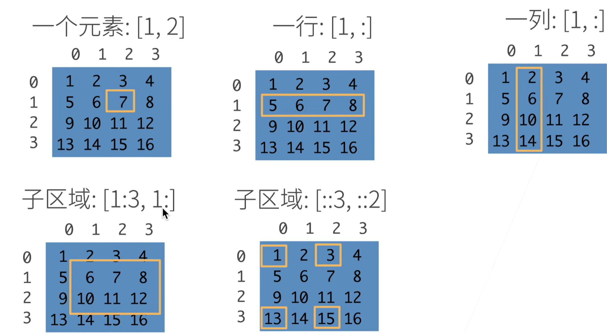
访问元素
x[row,column] 规则与列表切片相同
数据操作
1 | |
数据预处理
- 首先创建一个人工数据集作为例子
1 | |
- 接下来使用pandas读取生成的.csv文件
1 | |
终端会输出.csv文件的样式
1 | |
- 现在处理缺失数据
常用的方法包括插值和删除。这里使用插值。对于非数值的缺失值,我们可以选择将“NaN”视为一个类别。
下面是处理缺失值的代码:
1 | |
.iloc是pandas的索引器,通过位置选择数据(0:2表示选择前两列)。
.fillna方法用于填充缺失值,可以使用均值、中位数等替代NA值。
pd.get_dummies将分类变量转换为独热编码,dummy_na=True参数使NA值也被视为一个独立类别。
- 最后转换为张量格式
1 | |
pytorch使用
Dataset 和 Dataload 类
PyTorch中的Dataset和DataLoader类是数据加载和预处理的关键组件,它们能有效地处理各种类型的数据。
Dataset是抽象类,用于表示数据集,它有两种主要类型:
1 | |
DataLoader是对Dataset的包装,提供了批处理、打乱数据、并行加载等功能:
1 | |
Dataset可以与数据变换函数结合,实现数据增强:
1 | |
当批处理中的样本无法简单堆叠时,可以定义自定义收集函数:
1 | |
自动求导
PyTorch的自动求导系统是其核心功能之一,能够自动计算神经网络中所有参数的梯度,这对于梯度下降类的优化算法至关重要。
1 | |
自动求导系统需要注意几个关键点:
计算图:PyTorch构建动态计算图,记录操作历史,以便反向传播。
梯度累积:每次调用
.backward()会累积梯度,除非手动清零:
1
2
3
4optimizer.zero_grad() # 优化器方式
# 或
for param in model.parameters():
param.grad = None高阶梯度:PyTorch支持计算高阶导数:
1
2
3
4
5x = torch.tensor([1.0], requires_grad=True)
y = x**3
y.backward(create_graph=True) # 保留计算图以计算二阶导数
x.grad.backward() # 计算二阶导数
print(f'二阶导数: {x.grad.grad}') # 应为6.0矢量计算加速:自动求导系统针对矢量运算进行了优化,所以通常应避免使用Python for循环。
线性神经网络
线性回归
样本(sample):每行数据
标签(label):预测的目标
特征(feature):预测依据的自变量
一般通常使用n来表示数据集的样本数。对索引为i的样本,其输入表示为x(i) = [x1(i), x2(i)]T,其对应的标签为y(i)。
线性回归模型
有两个假设:
假设一:影响预测目标的有几个关键因素,记为x1, x2, x3
假设二:预测目标是关键因素的加权和:y = w1x1 + w2x2 + w3x3 + b
用向量表示就是:
给定一个n维输入:x = [x1, x2, ..., xn]T
线性模型有一个n维权重和一个标量偏差:w = [w1, w2, ..., wn], b
输出时输入的加权和:y = < w, x > +b
线性模型可以看做是单层线性网络。
损失函数
我们通过损失函数来衡量预估质量
假设y是真实值,ŷ是估计值,我们可以比较:
这个叫做平方损失
代入求解可以得到训练损失函数为:
我们这里就要最小化损失来学习参数
基础优化方法
梯度下降
当没有办法求出解析解的时候,就可以使用梯度下降的方法来优化
挑选一个初始值 w0
重复迭代参数 t=1,2,3
沿梯度方向将增加损失函数值
学习率:步长的超参数。学习率不能太小,也不能太大。太小会导致梯度下降轮次过多,太大会导致函数震荡无法逼近最优解。
小批量随机梯度下降
在整个训练集上做梯度下降耗费时间太长。一般选择随机采样b个样本来近似损失。
b是批量大小,是一个重要的超参数。
梯度下降就是不断沿着梯度反方向更新参数求解;
小批量随机梯度下降是深度学习默认的求解算法;
两个重要的超参数是批量大小和学习率
从零构建线性回归
1 | |
用框架构建线性回归
1 | |
softmax回归
softmax回归其实是分类问题。回归估计一个连续值,分类预测一个离散类别